Iris Data Experiments

This notebook runs the experiments and generates the figures on the Iris data set.

import numpy as np
import pandas as pd
import seaborn as sns
import matplotlib.colors as mcolors
import matplotlib.pyplot as plt
import warnings
import itertools as it

# our code packaged for easy use
import detect_simpsons_paradox as dsp

iris_df = pd.read_csv('../../../data/iris.csv')
iris_df.head()

	sepal length	sepal width	petal length	petal width	class
0	5.1	3.5	1.4	0.2	Iris-setosa
1	4.9	3.0	1.4	0.2	Iris-setosa
2	4.7	3.2	1.3	0.2	Iris-setosa
3	4.6	3.1	1.5	0.2	Iris-setosa
4	5.0	3.6	1.4	0.2	Iris-setosa

From examining the above, we know that the class is the group-by variables and the float type variables are the continuous attributes. First we select the columns accordingly and output the names of the selected columns of each type to verify.

groupbyAttrs = iris_df.select_dtypes(include=['object'])
groupbyAttrs_labels = list(groupbyAttrs)
print(groupbyAttrs_labels)

['class']

continuousAttrs = iris_df.select_dtypes(include=['float64'])
continuousAttrs_labels = list(continuousAttrs)
print(continuousAttrs_labels)

['sepal length', 'sepal width', 'petal length', 'petal width']

Results

Now we can run our algorithm and print out the results after a little bit of post-processing to improve readability.

# run detection algorithm
result_df = dsp.detect_simpsons_paradox(iris_df)

# Map attribute index to attribute name
result_df['attr1'] = result_df['attr1'].map(lambda x:continuousAttrs_labels[x])
result_df['attr2'] = result_df['attr2'].map(lambda x:continuousAttrs_labels[x])
# sort for easy reading
result_df = result_df.sort_values(['attr1', 'attr2'], ascending=[1, 1])

result_df

	allCorr	attr1	attr2	reverseCorr	groupbyAttr	subgroup
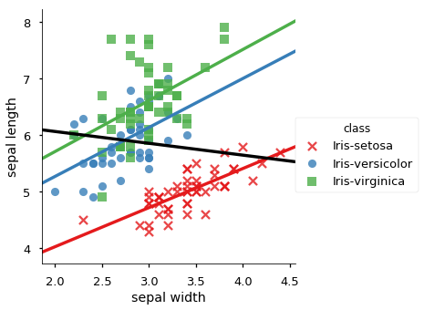
0	-0.109369	sepal length	sepal width	0.746780	class	Iris-setosa
3	-0.109369	sepal length	sepal width	0.525911	class	Iris-versicolor
6	-0.109369	sepal length	sepal width	0.457228	class	Iris-virginica
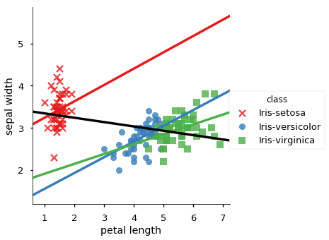
1	-0.420516	sepal width	petal length	0.176695	class	Iris-setosa
4	-0.420516	sepal width	petal length	0.560522	class	Iris-versicolor
7	-0.420516	sepal width	petal length	0.401045	class	Iris-virginica
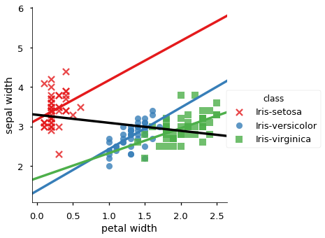
2	-0.356544	sepal width	petal width	0.279973	class	Iris-setosa
5	-0.356544	sepal width	petal width	0.663999	class	Iris-versicolor
8	-0.356544	sepal width	petal width	0.537728	class	Iris-virginica

Plotting

We plot all data in scatter plots based on each group by attribute, for each pair of candidate attributes. For each plot we add the overall trendline and the trend line for each occurence of Simpson’s Paradox.

Plotting with data frame

Plots in simpler code

# create a set (to keep only unique) or the attribute pairs that had SP
sns.set_context("talk")
sp_meas = set([(a,b) for a,b in zip(list(result_df['attr1']), result_df['attr2'])])
# for x,y in it.combinations(measurements,2):
for x, y in sp_meas:
    sns.lmplot(y,x, data=iris_df, hue='class', ci=None,
               markers =['x','o','s'], palette="Set1")
    # adda whole data regression line, but don't cover the scatter data
    sns.regplot(y,x, data=iris_df, color='black', scatter=False, ci=None)

Experiments on subsampled data

We run our algorithm on 10%, 30%, 50%, 60%, 90% sampled data set with 5 random repeats and for each couont the number of detections.

portions = [.1,.3, .5, .6, .9]
num_repeats = 5

# for sampling
rows = []
iris_df_portion = []
res_df = dsp.detect_simpsons_paradox(iris_df)
res_df['portion'] = 1
res_df['exp'] = 0


summary_cols = ['portion', 'exp', 'SPcount']
summary_data = [[1,0,len(res_df)]]


for i,cur_portion in enumerate(np.repeat(portions,num_repeats)):
    # sample and run detector algorithm
    res_tmp = dsp.detect_simpsons_paradox(iris_df.sample(frac=cur_portion))
    # append results with info on this trial
    res_tmp['portion'] = cur_portion
    res_tmp['exp'] = i +1
    res_df = res_df.append(res_tmp)
    summary_data.append([cur_portion, i, len(res_tmp)])

# make a dataframe of the summary stats
summary_df = pd.DataFrame(data =summary_data, columns =summary_cols)

Now, we can compute descriptive statistics on the occurences summary, using the grouby feature

exp_summary = summary_df.groupby('portion')['SPcount'].describe()
# exp_summary.count()
# summary_df
exp_summary

	count	mean	std	min	25%	50%	75%	max
portion
0.1	5.0	6.2	1.788854	4.0	6.0	6.0	6.0	9.0
0.3	5.0	9.0	0.707107	8.0	9.0	9.0	9.0	10.0
0.5	5.0	9.0	0.000000	9.0	9.0	9.0	9.0	9.0
0.6	5.0	8.8	0.447214	8.0	9.0	9.0	9.0	9.0
0.9	5.0	9.0	0.000000	9.0	9.0	9.0	9.0	9.0
1.0	1.0	9.0	NaN	9.0	9.0	9.0	9.0	9.0